For a correct modelling of the joints between segments in a TBM tunnel
2. (Part 1)Joints within the same rings (longitudinal joints)
3. (Part 2) Non-linear analysis
Click here to see the on-demand webinar
3. Non-linear analysis
Let’s imagine studying the installation of the ring and its annular gap filling to double check the crack patterns and the ovalisation (the lack of circular shape). In this case the stresses in the steel of the re-bars, could reach values up to 400 MPa, when cutting the steel bar. Indeed, it is worth pointing out that a kinematic model of the structure shows how a small angle offset (0.5%) at one joint during ring installation results in a displacement equal to 45mm, e.g 0.4% of the inner diameter.
In non-linear analysis the segments are modelled as non-linear frame elements, while the back-filling material is modelled by means of linear springs. The joints between segments have been simulated as non-linear frame elements with a section of steel at the middle of the cross section.
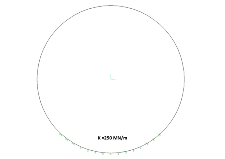
Figure 5. Non linear model
The structural elements considered in the analysis have the following geometrical characteristics and uncracked mechanical properties:
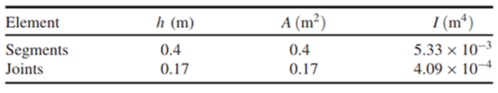
Table 1. Geometrical characteristics and gross mechanical properties of structural elements
In order to limit the deformations, the extension of the saddle (usually measured in degrees) takes on a fundamental importance in the problem definition. In fact, the greater the extension of the saddle area, in phase 1 of Figure 1, the smaller the displacements which appear along the ring.
.%20Bolts%20are%20visible%20between%20segments.png?width=726&name=Figure%206%20Ring%20saddle%20(80%C2%BA,%20split%20in%20in%2040%C2%B0+40%C2%B0).%20Bolts%20are%20visible%20between%20segments.png)
Figure 6 Ring saddle (80º, split in in 40°+40°). Bolts are visible between segments
Figure 6 shows the positions of longitudinal bolts whose main function is to “close” and ensure proper ring geometry of the ring from phase 1 to phase 3 of Figure 1.
The project, object of this study, provided a theoretical extension of saddle zone of 80º divided in two symmetric portions of 40º, as shown in Figure 6. The first step in the analysis was to recreate the theoretical conditions. The length of the saddle ring zone has been modelled using vertical springs. The springs can be derived from the subgrade modulus
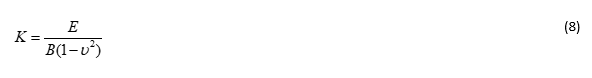
Formula based on Galerkin approach (see Bowels 1997)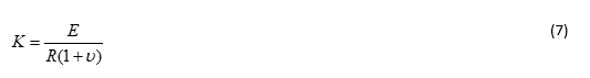
where: K= subgrade modulus, E= Young modulus of the soil., R= radius of the tunnel (5.57m), ν= Poisson ratio (0.2)
Formula by Bowels, based on Vesic´s approach (see always Bowles, 1997)
where: E= Young modulus of the soil, B= equivalent foundation width [see for instance page 509 of Bowles, 1997, ν= Poisson ratio
To evaluate the equivalent subgrade modulus along the saddle area, three different hypotheses were made.
- The subgrade modulus is a function only of the mortar Young´s modulus (evaluated 30GPa). The thickness of the mortar is 0.125m which is the gap between the rear of the TBM and the surface of the lining.
- The subgrade modulus is a function of the mortar and that of underlying soil. The thickness of the equivalent layer is 0.25m which is two times the gap thickness. Each layer is considered with a depth of 0.125 m
- The subgrade modulus is a function of the Young´s modulus of the mortar and that of the underlying soil. The thickness of the equivalent layer is 1.5m which is 12 times the gap extension. The mortar layer is 0.125m deep and the underlying soil is 1.375m.
Each of three hypotheses was examined using both Galerkin´s and Bowels´ approach. In summary 6 calculations were made. Following Bowels 1997, the Young modulus for a layered soil can be expressed as:
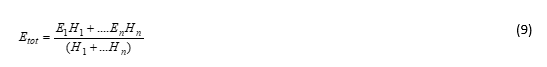
where: Etot= layered Young´s modulus, E1…En= Young´s modulus of layer 1…n, H1…Hn= thickness of layer 1…n
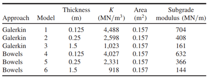
Table 2 Different Sub-grade Scenarios
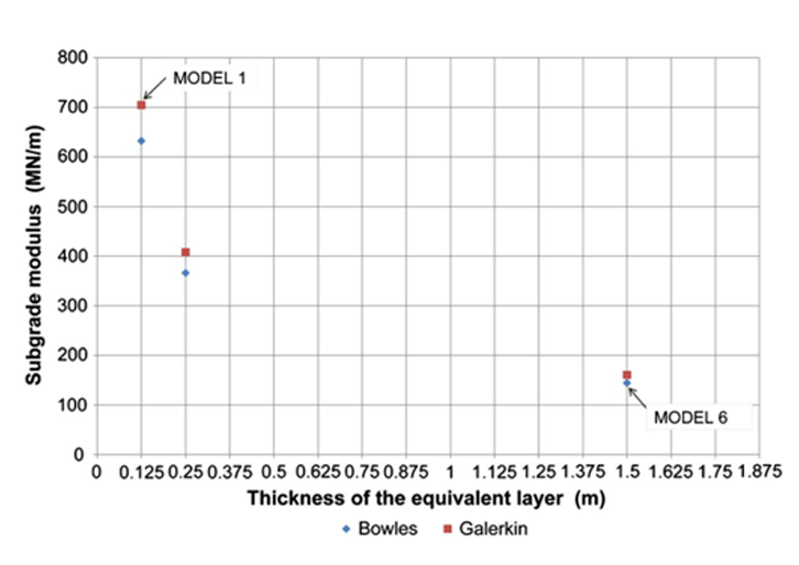
Figure 7 Sub-grade Moduli Variation
Once the subgrade moduli have been obtained for each one of the six possible combinations, each value has been multiplied by the equivalent frame area (0.157m) and the subgrade modulus, for each frame, has been obtained as shown in Figure 7, where it is possible to see how the difference between the various subgrade moduli can be six times (model 1 / model 6).
Table 2 collects all the subgrade moduli employed in non-linear calibrations. Figure 7 shows the relation between thickness of the equivalent layer and the subgrade modulus. Model 1, for example, corresponds to subgrade modulus following Galerkin´s approach with an equivalent thickness of 0.125 m while model 6 corresponds to Bowles´s approach with an equivalent thickness of 1.5m.
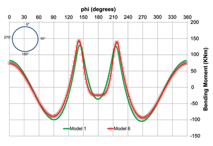
Figure 8. Relation of Bending moment depending of the models employed
Figure 8 shows the values of the bending moments as function of the tunnel angle (0° at crown and 180° at invert arch) for the two different subgrade moduli (model 1 and model 6). It is possible to see how the difference in terms of bending moments is about 9% at the crown and 21% at invert arch. These differences are rather small, in spite of the significant difference in the value of the subgrade modulus.
It was finally decided to employ a value of subgrade modulus equal to 250 MN/m, because, within the estimated range, it better simulates the plastic zone around the tunnel. The model is shown in the Figure 9 :
%20vs%20real%20ring%20(at%20left).png?width=726&name=Figure%209%20Model%20employed%20in%20analysis%20(at%20right)%20vs%20real%20ring%20(at%20left).png)
Figure 9. Model employed in analysis (at right) vs real ring (at left)
As it is visible in Figure 9, two cross sections were employed:
- Cross section of the segment with a height of 0.40m of concrete and steel rebars
- Joint section, with a height of 0.17m and a steel bolt exactly at the centre of the section
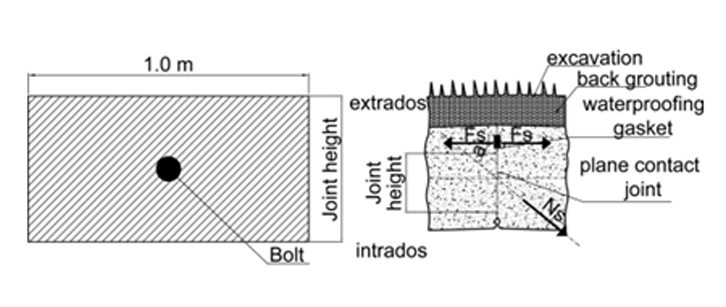
Figure 10. Joint section area
Each segment, in fact, is connected to the others along the longitudinal joint with two longitudinal bolts (along the same ring) and along the transverse joints also with transverse bolts (with the adjacent ring). Each bolt is 25 mm diameter with tensile strength of 1040 MPa and a length of 0.520 m. The insertion angle is 30º (Figure 10). Fd,n is fixed at 700 MPa. The joint section with the concrete in compression and the bolt in tension works as a rotational spring with elasto-plastic behavior.
It is important to underline that the main function of the bolts, mainly the one placed along the longitudinal joints, is to connect all the segments within the same ring, providing enough resistance to balance the ring´s self-weight in absence of a significant axial force.
This is the main reason why bolts must be taken into account during the verification of the construction phases. The bolts were modelled with a frame element whose cross section is shown in Figure 9 (left). Constitutive laws, with average values for concrete and steel bars have been employed.
The methodology of the analysis carried out is based on P’erez et al, 2012 and it consists in the following steps:
- First of all a linear analysis is carried out to determine the internal force envelopes along the ring.
- For each section of the model, the bending moment is compared to the yielding moment. The yielding moment has been evaluated as 128 KNm
- When the computed bending moment is greater to than the value established for yielding (128KNm), a hinge is considered to be formed at that location, carrying a bending moment equal to this value. In this way, internal forces redistribute along the ring. This artifice allows to reproducing the r response of a structure under bending moments when yielding is reached.
- This process has to be repeated until bending moments within the ring are less than the yielding moment or until the structure has collapsed (formation of 5 plastic hinges).
Three scenarios have been reproduced varying the extension of the saddle area as shown in Figure 11.
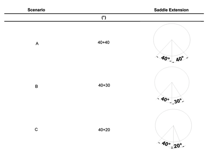
Figure 11 Scenarios analyzed depending of the saddle extension
The results of the models are shown in Table 3 where it is possible to check the evolution of the internal force redistribution when a hinge is inserted in the model. Model “A” reaches a maximum crack width of 0.3 mm and the ovalisation seems to be constant with a value of 13mm. Model B reaches a maximum crack value of 1.0 mm at the tunnel crown while the ovalisation increases from 17.0 mm with model “B1” to 56.0 mm with model “B3”.
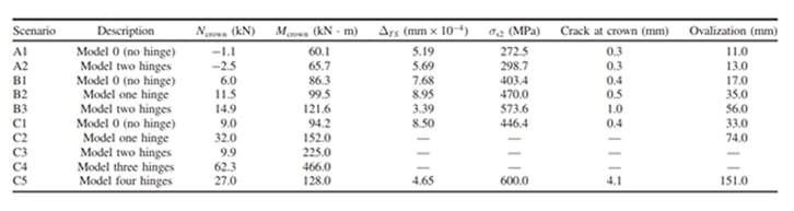
Table 3. Summary table among the different scenarios and their evolution after the redistribution steps
Model C assumes the formation of a series of hinges, during the redistribution process, where the bending moment is higher than the moment producing yielding of the reinforcement one until “C5” where equilibrium is reached at all sections.
4. Conclusions
From the above discussions the following conclusions can be drawn:
| 1 |
The approach of tunnel design based on elastic behavior of reinforced concrete, while generally acceptable for service conditions, is not always adequate for the initial phase of ring installation, since the axial forces at the joints are very low. |
| 2 | For the construction phase the usual models (Jansenn, Blom) are not applicable due to lack of axial force. For this case, the analysis must take into account provisional bolts which guarantee the structural integrity during this phase. This analysis can be carried out in MIDAS GTS NX simulating the segments as shells with different thickness. |
| 3 | For the permanent phases the usual models (Jansenn, Blom) can be applicable because of the ground forces. These joins can be efficiently simulated in Midas GTS as interface with Jansenn formulation |
| 4 | During construction phase, it is important also to evaluate the asymmetrical configuration of the saddle because it can lead big values of ovalisation of the rings. |
The model employed, simulating the joints among the segments, allows to model hinges within the ring which lead to redistribution of internal forces. This redistribution capacity is the reason why the formation of a hinge within the ring does not lead to collapse.