For a correct modeling of the joints between segments in a TBM tunnel
2. (Part 1)Joints within the same rings (longitudinal joints)
3. (Part 2) Non-linear analysis
Click here to see the on-demand webinar
1. Introduction

A tunnel boring machine is a machine capable of excavating a tunnel with the complete cross section, and can be equipped, according to the different cases, with auxiliary modules for the positioning of provisional linings. The injection of the space between the ring and the ground (the so-called gap), created by the difference between the rear of the shield and the ring, is an element related more to the construction process of the tunnel than to design as stated in ITA, 1999 and ITAtech, 2014. Gap backfill is meant to perform several functions:
▪️ It ensures a uniform distribution of the ground pressures.
▪️ It reduces decompression of the ground that could have negative effects on subsidence
(in particular for superficial tunnels)
▪️ It works as an additional barrier for waterproofing.
▪️ The alkalinity of the contact between the ground and the lining increases,
so the durability of the ring improves.
(More information on gap back-fill can be found in references Cavalaro 2009 and Pelizza et al. 2010)

Figure 1. Gap filling phases carried out in the real case
Figure 1 shows the procedure of gap filling for tunnels in rock/soil. The phases of gap filling are:
- Phase 0: the ring has been installed and is held in place by longitudinal and circumferential bolts within the shield
- Phase 1: Execution of the so-called “saddle”. This operation starts just after the ring installation. The ring, at this stage, is outside the shield.
- Phase 2: Execution of the drift-walls gap filling. This operation takes some time to be covered and starts after the installation of 2 to 4 other rings.
- Phase 3: gap-filling completion. This operation takes place after the installation of another 2 to 4 rings
In summary, the time each ring has to “wait” before its gap is filled can vary from four to eight other ring installations. If the TBM advance does not encounter any problems (geological formation, local presence of water table) or any maintenance problems (cutters, convoy belt and so on), the time between phase 1 and phase 3 theoretically lasts from one to three days. During this time, the ring is experimenting deformations, which can alter its internal stress distribution.
The importance of simulating the joints between rings can be due to particular structural and geotechnical conditions as a more reliable assessment of the ring deflections, earthquake conditions and so on. In this blog we are going to focus our attention to the so-called longitudinal joints, defined as the joints between segments of the same ring because their modeling is more frequent.
2. Joints within the same rings (longitudinal joints)
The first studies on tunnel joints were carried out by Gladwell, 1980, and Jansenn,1983, based on the study of concrete joints carried out by Leonhardt and Riemann in 1966. Their idea was to simulate the contact between two segments, i.e. the joint, considering concrete as an elastic material and its contact as direct and uniform. In other words, they proposed to simulate the mechanism dowels/joint /segment as an equivalent beam made of three distinctive beams with a “finite” discontinuity as shown in Figure 2.

Figure 2. Jansenn´s Equivalent beam approach
This artifice allows simulating the joint rotation and its curvature using a beam of variable depth. If we refer to Jansenn’s approach it is possible to see how the linear relationship between bending moment, M, and joint rotation a function of the axial force is, N, and of the joint geometry:
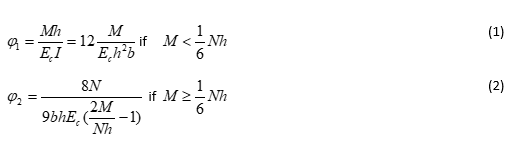
where:
h= joint height (m)
b= joint thickness (m)
Ec and I have the same definition employed for equation (1) and N, M are the internal forces (Axial load and bending Moment).
φ= joint rotation (radians)
This equation expresses the rotation (φ) of the joint in radians.
Jansenn´s approach is more accurate for thick joints because in the equivalent ‘beam’ a curvature will develop resulting in a rotation. In reality, when the joint is very thin, only a very minor additional rotation will occur. Because of the hypothesis that the joint has a length equal to the height of the joint, according to Janssen, a rotation will develop taken into account for the spread of load in the region of the joint.
Regarding this, the Janssen relation will be more accurate when describing a thick joint. Gladwell proposed another relationship Moment/joint rotation, which is very similar to the Janssen’s except for the introduction of the intrinsic properties (Ec and moreover Poisson ratio) of reinforced concrete. The formula is:
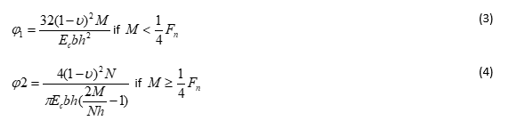
As shown by Van Der Vliet, 2010, and afterwards by Peña, 2012, there are three main differences between the Gladwell’s and Janssen’s approach:

Figure 3. Comparison between Jansenn and Gladwell approach for the studied case
- The initial stiffness obtained by Gladwell is greater than Janssen’s. This is due to the type of analysis carried out by Gladwell in which the contact stress is concentrated on the edges of the joint.
-
The non-linear branch proposed by Gladwell reaches very quickly the maximum theoretical bending moment because Gladwell´s approach stiffness is higher and the joint stayed close longer than Jansenn´s one (Figure 3).
- The differences encountered between the two solutions, in particular in the linear branch, are due to the different formulation of joint and the segment height.

Figure 4. Janssen’s law in Midas GTS NX
Van Der Vliet, 2010 showed that the joint simulation in finite element modelling, seems to better follow the Gladwell’s approach than Janssen’s if the structure is simulated as solid element, because it takes into account the mechanical properties of concrete (Ec and υ). In the engineering practice, however, the structure elements are usually simulated as beam/shell elements and they implement already the mechanical features of the elements; in this case the Janssen approach results more reliable in terms of numerical approach. This is the reason why in Midas GTS NX is possible to simulate the joints between segments as Janssen (see Figure 4)
In order to better simulate the joints in finite elements models, Blom, 2002 considered the longitudinal joints as flexural springs with stiffness, “cr”, defined as:
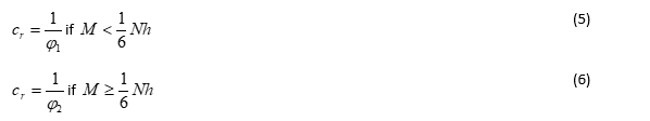
Where the terms φ1 and φ2 are those of equations (1) and (2). Equation 5 is employed when the rotational stiffness is non-linear but the ultimate compressive strains are in the elastic branch. The circumferential joints are considered as shear springs too. Arnau, 2012 has adopted this formulation in his experimental study with good results.
If we wanted to simulate the Blom criteria, in MIDAS GTS NX we have to create a “Node connection/rigid link”.'
These cited studies were carried out determining the stress distribution and deformation of an ovalised ring assuming three main hypotheses, which are not in fact realistic:
▪️ The ring is radially loaded,
▪️ The Gap between rock and lining is completely filled
▪️ Concrete ring behavior is always linear elastic
These hypotheses are not fulfilled in absence of a significant axial force or when the gap is not yet filled, for example during construction phases. In this case the only bending capacity to support the weight of the segment is provided by the longitudinal bolts.
The main issue in engineering practice is the magnitude of the deformation when the load is not radial, in the absence of a significant axial force acting on the ring, and when the ring, because of the lack of gap-fill is free to expand. In this case, the deformations and the stress distributions are completely out of range when comparison is made between the field data and those values calculated with the models available in technical literature and summarized above because all of them take into consideration that the ring is perfectly confined and immersed into the soil: in other words, the ring displacements would be very small.
It is, therefore, not possible to study these effects referring to the technical literature available. The new approach presented in this study is based on non-linear behavior of R.C. based on the constitutive laws of the materials which leads to a redistribution of the internal forces, in particular of bending moments, and considers provisional bolts which are actually responsible for the achievement of equilibrium in the unfavorable conditions typical of construction phases.
>> Click here to read the part 2
3. Non-linear analysis
4. Conclusion